Squamish Spit — ML forecast
Why this page exists
I’m a paraglider. I want to fly off the Stawamus Chief in Squamish, BC and land down in the valley. For most of the warmer half of the year that valley funnels a strong, consistent inflow wind up Howe Sound—a south breeze that the kiteboarders at the Squamish Spit live for and that paragliders generally cannot land in safely. Sustained 30–50+ km/h from the south at the Spit anemometer is normal on a sunny summer afternoon, and a wing on final into that is not where you want to be.
The frustrating part: public weather forecasts dramatically underpredict the Spit inflow. HRDPS, GFS, the consumer apps stacked on top of them—when it is really blowing on the beach, the gridded model wind is often about half of what the meter is reading, sometimes worse. Whatever the grid resolves at the head of Howe Sound is not what a sensitive 10 m anemometer at the Spit actually feels. Treating a generic forecast as a green light has burned a lot of Squamish pilots.
Flying the Chief takes effort. You drive to the trailhead, put a full kit on your back, hike up, and lay out at launch waiting for cycles. The familiar bad day: drive over, hike up, sit at launch watching the Spit windmeter tick along at 40 km/h hoping it eases before sunset, and eventually pack the wing back in and hike all the way back down. Often the inflow does die down in the last hour before sunset and a flying window opens. Often enough that waiting it out can pay off—not so reliably that it always does.
So I built this: a small machine-learning model that targets the Spit anemometer specifically and is trained to flag the days where the inflow either never really fires or, more commonly in summer, eases at sunset enough to fly. The aim is to reduce wasted hikes—fewer days you drive over for nothing—not to promise launchable conditions.
The Spit windmeter is the only real go/no-go
Once you are at launch and trying to decide whether to take off, the number that matters is the live Spit anemometer—not this forecast. WeatherFlow updates roughly every 5 minutes. If the meter says it is still blowing, you do not fly. Even if everything else, including this model, told you it would be calm by then. Squamish pilots routinely hike up, wait an hour, see no easing, and hike back down. That outcome is part of paragliding here. This page exists so you can have to do that fewer times—not so you can ignore the meter once you are already at the top.
What you see in the panel
Click the Spit marker on the map and a bottom panel opens with two strands:
- Live WeatherFlow. The current Spit anemometer plus the recent timeseries—mean speed, gust, lull, direction. This is the strand you read at launch. If it is still blowing, do not fly.
- ML wind forecast. Hour-by-hour mean wind speed (with a 68% uncertainty band) and direction for today and tomorrow in Pacific local time. This is the strand you read the night before, the morning of, and as you are deciding whether to commit to the drive and the hike.
A “Today / Tomorrow” toggle switches between them. The forecast JSON is served from /api/spit-forecast once the backend has run the hourly generator.
Today vs Tomorrow strand
The hourly job sets an issue hour t_cut_local_hour to the current local wall-clock hour. It runs the model once with today’s observations through hour t_cut − 1 visible and produces speeds and directions for the rest of the day (hours t_cut–23). It then runs a second pass for tomorrow with no station data (t_cut = 0 on a synthetic day), driven only by the latest HRDPS / marine forecast cycle. So today tightens through the day as real anemometer hours fill in, and tomorrow is the model’s pure forecast view—useful for “should I plan to drive to Squamish tomorrow?”
Each hour of the JSON gives you avg_p50 (the predictive median), an avg_ci68_lo / avg_ci68_hi band (~68% predictive interval interpolated from the trained quantiles), and wind_dir_deg. Gust and lull distributions are trained but the chart focuses on mean wind. The band represents model uncertainty—not a regulatory or official forecast interval.
How accurate is it on the days you care about?
All of the figures below are scored on held-out validation + test calendar days the model never saw during training (random split across the whole 2023–2026 archive timeline, fixed seed, ~207 days). They are the offline equivalent of “how well would this thing have called these days had it been running live then?”
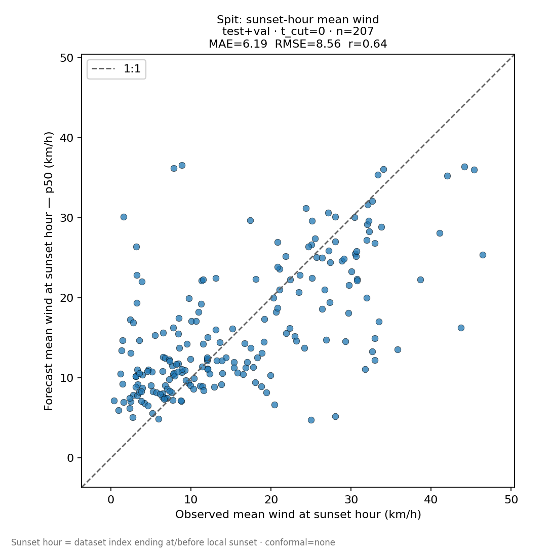
“Will sunset be flyable?” — the night-before view
For each held-out day, take the local hour bucket the dataset labels as “sunset” (the last full hour ending at or before astronomical sunset at the Spit), and compare the observed Spit mean wind in that hour to the model’s P50 mean-wind forecast. The forecast here is issued with no station data on that day (t_cut = 0)—essentially the same view as the tomorrow strand in the panel. Raw quantile head, no conformal adjustment.
“Should I leave for the trailhead?” — about two hours before sunset
From most parts of Squamish you can roughly drive to the Chief trailhead, hike up, lay out, and be ready to fly within about two hours of leaving the house. So the natural moment to commit is roughly two hours before the window you are aiming for. Same target hour at sunset, but the offline evaluation now lets the model see the day’s real Spit observations through t_cut = sunset_hour − 2. That extra context tightens the call.
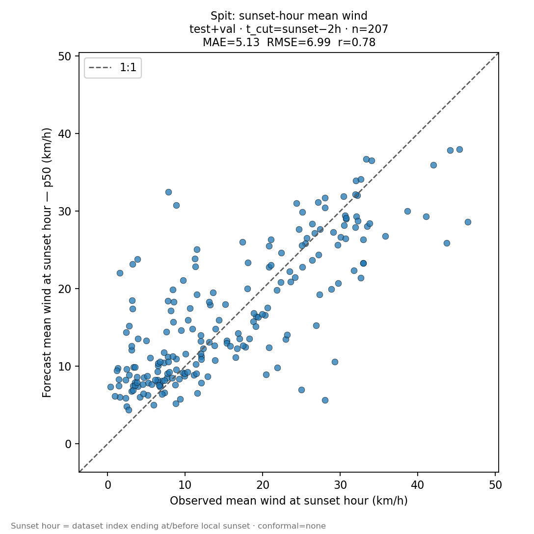
t_cut = 0 panel because the model is now anchored to the recent inflow trace. There is a small positive bias—the forecast tends to read a touch hot vs the meter at sunset. As a pilot rule of thumb: a P50 in the 25–30 km/h range at sunset usually means do not bother starting the hike; a P50 in the 10–15 km/h range with the band shrinking through the late afternoon is the kind of evening that more often opens a window. None of that overrides the live windmeter once you are up there.“Is it even an inflow day?”
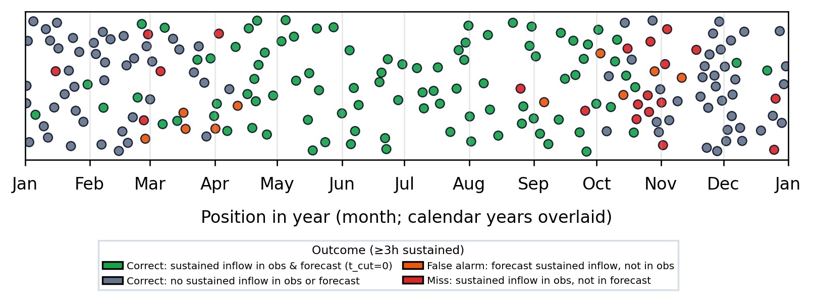
The mean-wind scatters tell you about a single hour. A coarser, more decision-flavoured question is: is this calendar day going to be an inflow day at all? The model is scored against the meter on a yes/no basis. A day counts as inflow if at least three consecutive local hours each have observed mean speed above about 20 km/h and direction in the south sector (140°–220°, ±40° around due-south). The forecast applies the same streak rule on conformal-adjusted quantiles. Evaluation is again at t_cut = 0, so this is the strict “tomorrow”-style check—no station replay.
How strong does it actually get on inflow days?
When the model and the station both classify a day as inflow, the next question is how hard it really blew. Each true-positive day is one pair: peak observed mean wind across hours where the station is reporting (wf_valid_frac ≥ 0.5) versus peak forecast P50 across the same eligible hours. The grey points are the same comparison but for raw HRDPS 10 m wind at Feather Park over those hours—the gridded model alone, no ML on top.
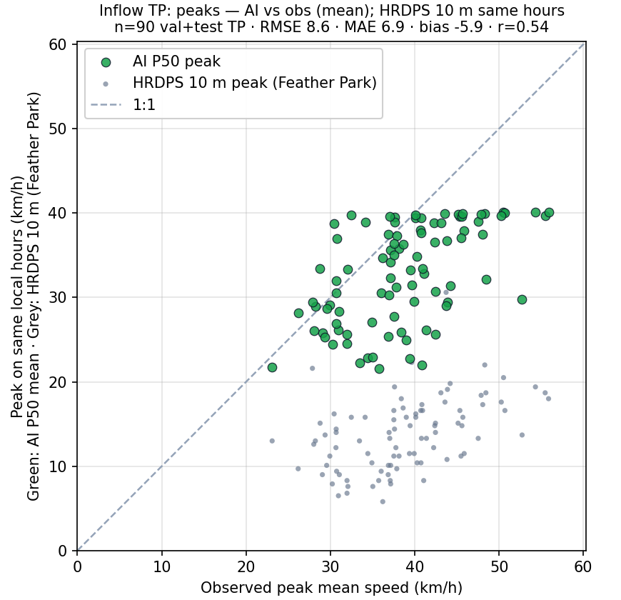
Why HRDPS alone isn’t enough at the Spit
Already implied above, worth stating outright. The continental HRDPS (~2–3 km grid) that the public Open-Meteo endpoint serves does not reproduce what the Spit anemometer measures—on strong inflow days it is often about half of the real wind. HRDPS West (~1 km) does measurably better, but it is still not a calibrated point forecast for the Spit and still tends to under-call honking days. Stacking ML on top of the grid is one way to bridge that gap; it is also why the live panel does not just plot the grid wind verbatim.
Under the hood
Model type
The core model is a small neural net called SpitBiGRU: a bidirectional GRU over the 24 local hours of one calendar day, with learned layers on top. It is trained with quantile loss on three speed channels—mean (average), gust, and lull—so each hour has a full predictive distribution, not a single number. A separate head predicts wind direction as a unit vector (sin/cos), converted to degrees for display. Optional conformal calibration can adjust speed quantiles before export so the uncertainty bands match recent residuals.
Inputs and data sources (live run)
Each forecast run builds a 24-row “virtual day” for today and tomorrow in Pacific local time, aligned with training:
- HRDPS (Open-Meteo) at fixed training grid points: Spit, Cloudburst (Whistler-area mountain), and Pemberton, each with the same fixed column template (surface winds and thermodynamics, cloud layers, boundary-layer / freezing-level heights, selected pressure-level winds and temperatures)—the list used in training and live pulls, not an arbitrary subset of the model grid or a GRIB dump.
- Marine analysis/forecast (e.g. Pam Rocks) for sea-surface temperature and mean sea-level pressure when available.
- Engineered scalars derived from those grids—valley-axis wind alignment, Pemberton minus Spit surface pressure difference (the classic “pressure gap” that drives the inflow), vertical wind shear at Spit (925 vs 850 hPa, 850 vs 10 m), the hourly change in that pressure gap, alignment of Pemberton vs Spit wind at 925 hPa, and parcel max buoyancy summaries from the Spit and mountain profiles.
- WeatherFlow station replay at the Spit: for each hour the model sees the same five channels used in training—mean, gust, lull, and direction (sin/cos). For “future” hours after the issue time, station inputs are masked out so the net must rely on NWP + marine + engineered features; short-term trends in the last few observed hours (slopes, direction change) are also fed in so the model is not limited to snapshot persistence.
Offline, the network was trained from a long archive: historical WeatherFlow CSVs + HRDPS day files + marine merged into a single Parquet dataset—one row per local hour for each joint calendar day where Spit WeatherFlow overlaps Spit and Cloudburst HRDPS. A representative build checked in for this project contains 937 such days (Oct 2023–Apr 2026). Training defaults in train_spit_forecast.py hold out validation and test calendar days at random across the whole timeline (fixed RNG seed), so scores are not dominated by one season the way a contiguous “last N months” tail would be; expected sizes for those defaults are about 730 training days, 92 validation, and 115 test. A chronological window split remains available via --data-split chronological. How far back the merged table can run is limited mainly by HRDPS historical-forecast availability from Open-Meteo (reforecast-style continental HRDPS): days before usable hourly fields exist at the archive grid points cannot enter the joint set, regardless of WeatherFlow logs. Inputs are standardized with coefficients stored in the model checkpoint so live rows use the same scaling.
Which variables matter most (permutation importance)
Research tooling measures “importance” by shuffling blocks of inputs (or single columns) and seeing how much offline scores worsen versus an unshuffled baseline—larger worsening usually means the model relied more on that signal. On validation days spread across the training timeline, the ranking was broadly:
- WeatherFlow observations (mean, gust, lull, direction)—by far the strongest block whenever those hours are visible; they anchor the forecast to reality.
- Spit HRDPS — especially 10 m wind speed, 925 and 850 hPa winds, 10 m gust, cloud cover, and boundary-layer height.
- Engineered pressure gap — Pemberton minus Spit surface pressure and its hour-to-hour change rank high among scalars; this matches the physical story that the Spit inflow is driven by the pressure gradient up the valley.
- Parcel max buoyancy (Spit and mountain) — moderate lift.
- Marine fields — small but efficient (only two columns).
- Pemberton HRDPS — valley / upstream context in the same HRDPS template as the other sites; block importance is usually smaller than Spit but not stripped down to a hand-picked subset of columns.
- Cloudburst HRDPS — mountain-side cloud layers, winds, and thermodynamics; marginal single-column scores often emphasize clouds and wind direction aloft.
Engineered calendar scalars (day-of-year and hour-of-day harmonics, daylight-related terms) supplement the hour sequence. Importance scores depend on the metric, season, and exact model revision; treat this list as engineering intuition, not a physical law.
Limits and safety
The ML layer sits on top of numerical weather prediction and a single anemometer. It will be wrong whenever the underlying models are wrong, when the station drifts or has a bad cell day, or when the Spit flow is dominated by something the grid does not resolve. Squamish-specific things it can miss include sudden marine push events, thunderstorm outflows, north outflow turning on early in shoulder seasons, and unusual stratification.
For paragliding the Chief, please remember:
- The model is a planning aid for “is it worth even trying today?”—not a launch decision.
- The live Spit windmeter at the time you intend to launch is the actual go/no-go. If it is still blowing, do not fly.
- The Chief is a different site from the Spit. Wind on the rock can differ from wind on the beach—exposure, lee, thermal interaction. Watch your launch and the air you can see (lake, water, vegetation, other pilots, kiteboarders) at least as carefully as any number on a screen.
- This forecast does not replace EC/U.S. public forecasts, local club rules, instructor input, or your own judgment.
Extra: what does the Spit normally do?
These plots summarize station-only history from the per-day Spit WeatherFlow archive—they are not inputs to the live forecast JSON. Useful background for pilots: how often does the Spit blow, when does it ease, and how reliably does it die for sunset.
How often is it calm in the last minutes before sunset?
For each local calendar day, take every archive sample whose timestamp falls in the last 15 minutes before astronomical sunset at the Spit (same latitude/longitude as the training grid). The day counts as “calm pre-sunset” if the maximum gust in that window is below 20 km/h. Days with no samples in the window are omitted. The curve pools many years onto a 366-day template (month–day, leap-year layout), then shows a 50-day wrapped rolling mean so early January smooths with late December. Read this as the climatological share of days when “wait it out for sunset” actually pays off at the meter.
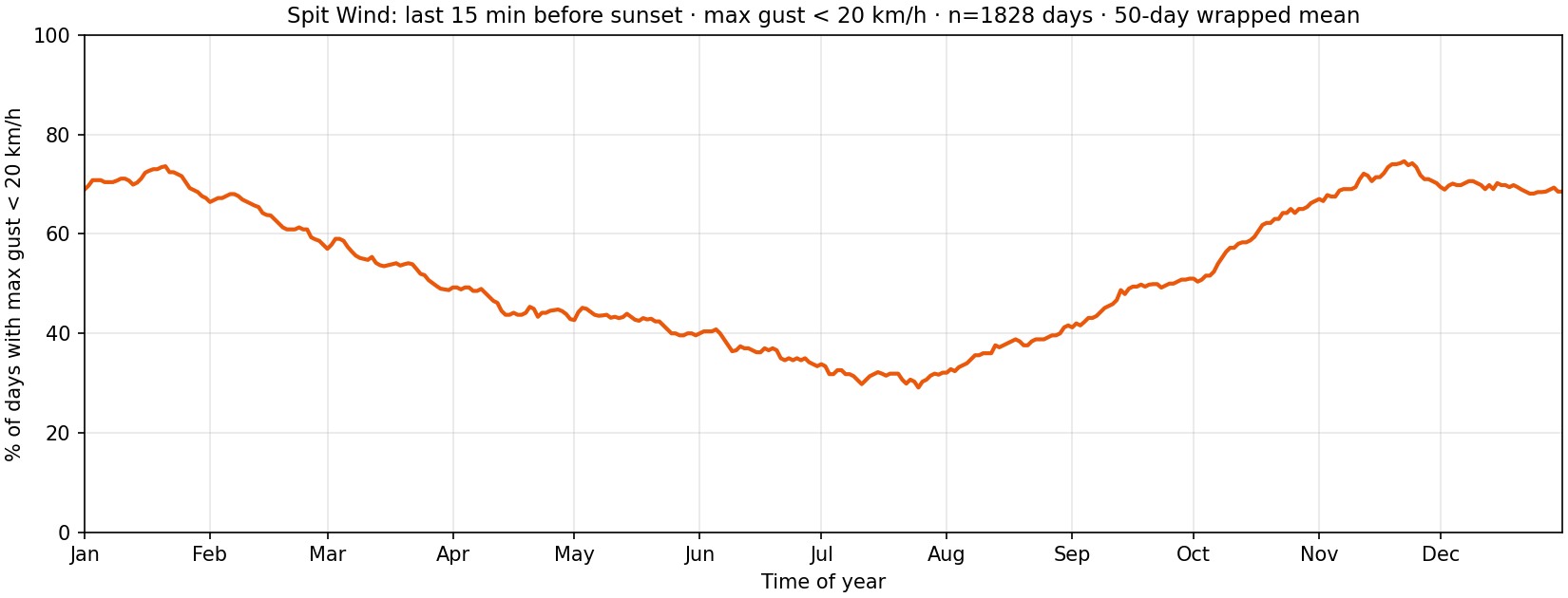
plot_pre_sunset_gust_seasonal.py on the Spit WeatherFlow CSV archive. Example snapshot: 1828 days with data in the window, ~52% calm overall.How hard does it usually get?
For each local day in the archive, bucket rows by clock hour. In every hour the gust samples are averaged into that hour’s bin. The day’s scalar is the maximum of those hourly means—i.e. the strongest hourly-mean gust that day (days need at least 18 hours with at least one gust sample). For each calendar month–day, the curve shows the mean of that scalar across years, then a 50-day wrapped rolling mean.
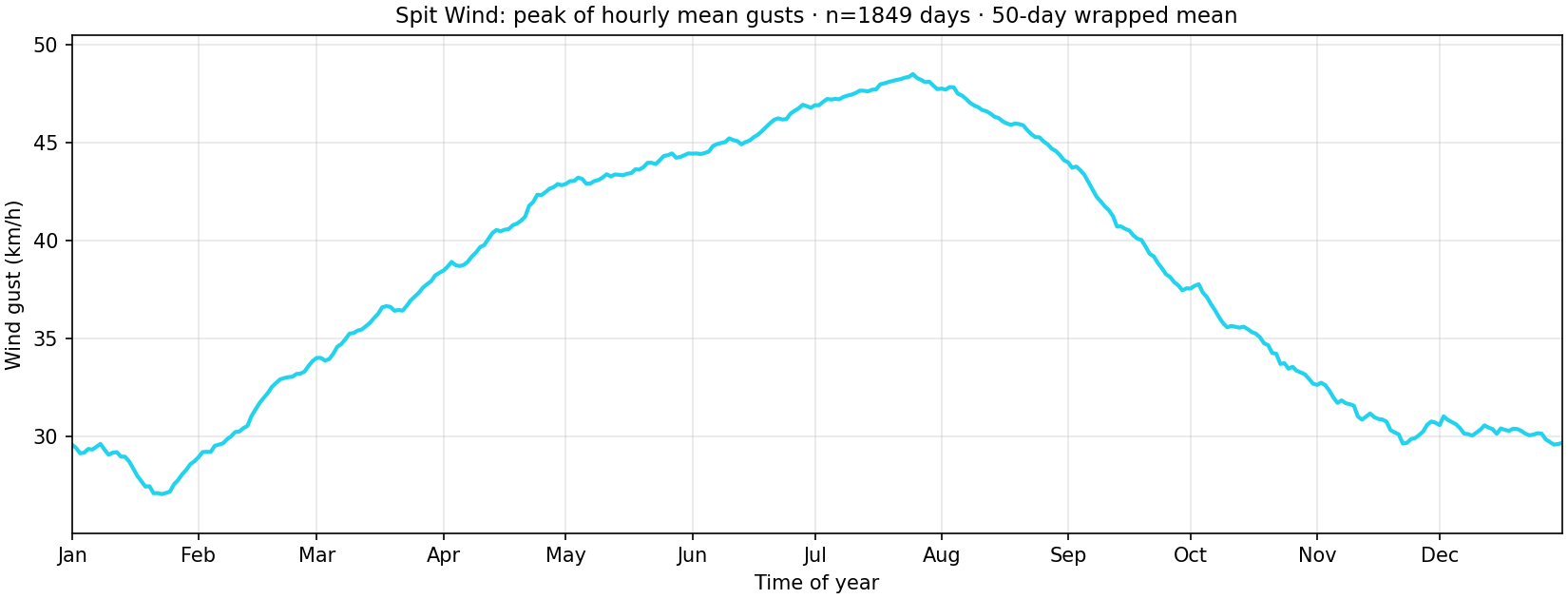
plot_hourly_peak_wind_seasonal.py (default --metric peak-hourly-mean). Example snapshot: 1849 days, overall mean of the daily metric ≈ 38 km/h.How often is it an inflow day in the first place?
Same observed inflow rule as the accuracy figure earlier on this page: a day counts if at least three consecutive local hours have aggregated station mean speed above 20 km/h and direction in the south sector (±40° around due-south, i.e. ~140°–220°), with hourly buckets requiring at least half their expected 10-minute slots populated. Days with no usable hourly truth are omitted.
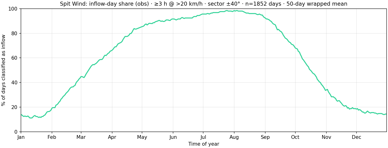
plot_inflow_day_fraction_seasonal.py. Example snapshot: 1852 labeled days, ~61% inflow overall; summer dominates, winter least. Practical translation: in the warmer months, the default expectation is that the valley is going to blow—the question is whether it eases enough at the end of the day to fly.When does the inflow normally start and stop?
For days that qualify as inflow, take the longest consecutive run of qualifying hours (earliest run if tied). Mean start is the average local clock hour the run begins (first qualifying hour). Mean end is the average first clock hour after the run (half-open: a run through hour 12 ends at 13:00). Same 366-day pooling and 50-day wrapped rolling mean.
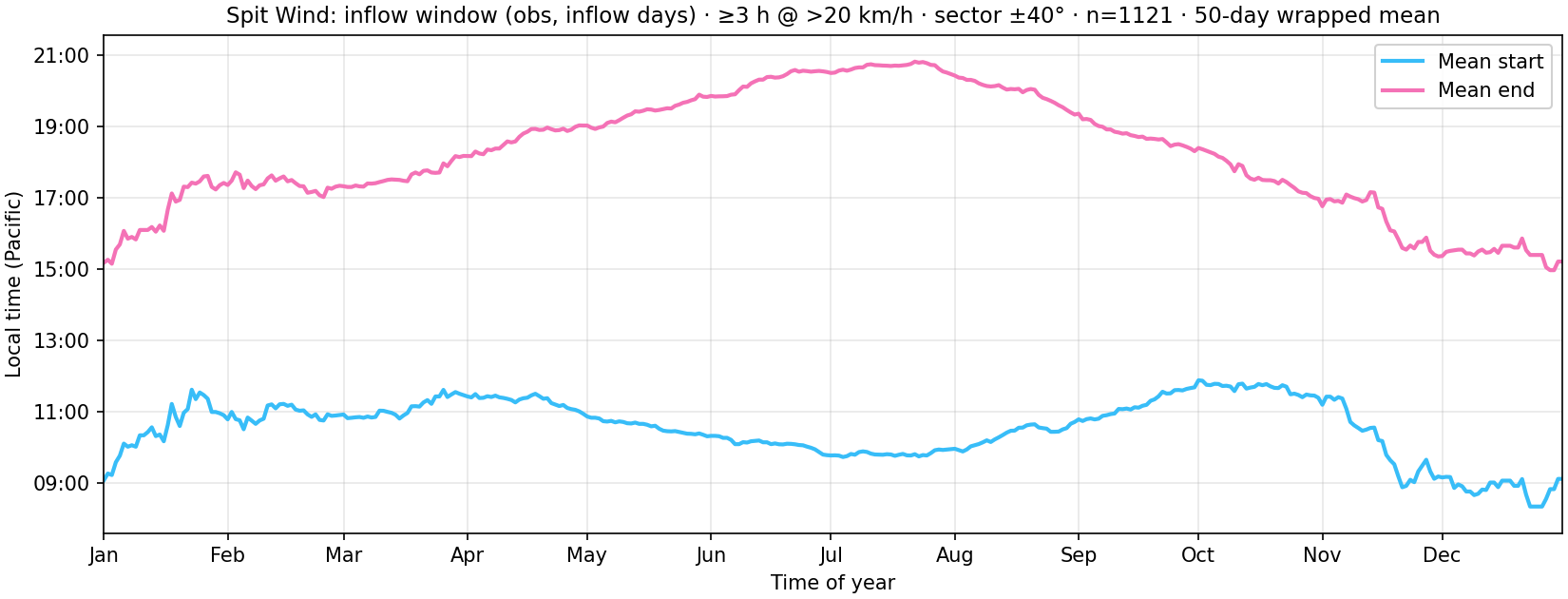
plot_inflow_start_end_seasonal.py. Example snapshot: 1121 inflow days, overall mean start ~10:37 and mean end ~19:07 Pacific. The end-of-day curve is the climatological hint that the inflow tends to stop late afternoon / early evening—the window the “wait it out for sunset” strategy is built on.Disclaimer. This page describes a planning aid for paragliders thinking about flying the Stawamus Chief and landing in the Squamish valley. It is not flying instruction. The live Spit windmeter at launch is the only real go/no-go—not this forecast, not any forecast. Weather, models, and instruments can all be wrong. You alone are responsible for your decisions.